Inspect

(Notebooke only) Interactive exploration of trained encoder and embeddings

import os
assert False == os.path.isdir('/app/data'), "Do not try to run this on solveit. The memory requirements will crash the VM."

import torch
import torch.nn.functional as F 
from torch.utils.data import DataLoader
from omegaconf import OmegaConf
import matplotlib.pyplot as plt
from PIL import Image
from IPython.display import display
import plotly.io as pio
pio.renderers.default = 'notebook'
from tqdm.auto import tqdm 

from midi_rae.data import PRPairDataset, ShiftedTripletDataset, TARGET_NAMES, SCHEME_NAMES
from midi_rae.vit import ViTEncoder, ViTDecoder
from midi_rae.swin import SwinEncoder, SwinDecoder
from midi_rae.utils import load_checkpoint
from midi_rae.viz import make_emb_viz, viz_mae_recon, show_fig_table

Config

#cfg = OmegaConf.load('../configs/config.yaml')
cfg = OmegaConf.load('../configs/config_swin.yaml')
#device = 'cuda' if torch.cuda.is_available() else 'mps' if torch.backends.mps.is_available() else 'cpu'
device = 'cpu'  # leave GPU free for training while we do analysis here.
print(f'device = {device}')

device = cpu

Load Dataset

#val_ds = PRPairDataset(image_dataset_dir=cfg.data.path, split='val', max_shift_x=cfg.training.max_shift_x, max_shift_y=cfg.training.max_shift_y)
val_ds = ShiftedTripletDataset(image_dataset_dir=cfg.data.path, split='val', max_shift_x=cfg.training.max_shift_x, max_shift_y=cfg.training.max_shift_y)

val_dl = DataLoader(val_ds, batch_size=cfg.training.batch_size, num_workers=4, drop_last=True)
print(f'Loaded {len(val_ds)} validation samples, batch_size = {cfg.training.batch_size}')

Loading 91 val files from /home/shawley/datasets/POP909_images_basic... Finished loading.
Loaded 9100 validation samples, batch_size = 370

Inspect Data

batch = next(iter(val_dl))
img1, img2, deltas, file_idx = batch['img1'].to(device), batch['img2'].to(device), batch['deltas'].to(device), batch['file_idx'].to(device)
print("img1.shape, deltas.shape, file_idx.shape =",tuple(img1.shape), tuple(deltas.shape), tuple(file_idx.shape))

img1.shape, deltas.shape, file_idx.shape = (370, 1, 128, 128) (370, 2, 2) (370,)

# Show a sample image pair
idx = 0
fig, axes = plt.subplots(1, 2, figsize=(8, 4))
axes[0].imshow(img1[idx, 0].cpu(), cmap='gray')
axes[0].set_title(f'Image 1 (file_idx={file_idx[idx].item()})')
axes[1].imshow(img2[idx, 0].cpu(), cmap='gray')
axes[1].set_title(f'Image 2 (deltas = {deltas[idx].cpu().int().numpy()})')
plt.tight_layout()
plt.show()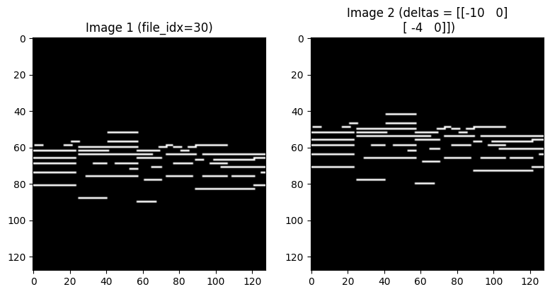

Load Encoder from Checkpoint

if cfg.model.get('encoder', 'vit') == 'swin':
    encoder = SwinEncoder(img_height=cfg.data.image_size, img_width=cfg.data.image_size,
                    patch_h=cfg.model.patch_h, patch_w=cfg.model.patch_w,
                    embed_dim=cfg.model.embed_dim, depths=cfg.model.depths,
                    num_heads=cfg.model.num_heads, window_size=cfg.model.window_size,
                    mlp_ratio=cfg.model.mlp_ratio, drop_path_rate=cfg.model.drop_path_rate).to(device)
else:
    encoder = ViTEncoder(cfg.data.in_channels, cfg.data.image_size, cfg.model.patch_size,
                         cfg.model.dim, cfg.model.depth, cfg.model.heads).to(device)
#encoder = load_checkpoint(encoder, cfg.get('encoder_ckpt', f'../checkpoints/{encoder.__class__.__name__}__best.pt'))
encoder = load_checkpoint(encoder, '../checkpoints/SwinEncoder_NoSim_best.pt')

encoder.eval()
print(f"Loaded {encoder.__class__.__name__}")

>>> Loaded SwinEncoder checkpoint from ../checkpoints/SwinEncoder_NoSim_best.pt
Loaded SwinEncoder

Run Batch Through Encoder

with torch.no_grad():
    with torch.autocast(device_type=device, dtype=torch.bfloat16):
        enc_out1 = encoder(img1)
        enc_out2 = encoder(img2)

Visualize Embeddings

NOTE: This will visualize all embeddings in the entire batch, not just the single pair of images shown above.

figs = make_emb_viz((enc_out1, enc_out2), encoder=encoder, batch=batch, do_umap=False)
show_fig_table(figs)

SVD Analysis

def svd_analysis(enc_out, level=1,  title='', top_k=20):
    "Run SVD on encoder output, plot singular value spectrum and cumulative variance"
    z = enc_out.patches[level].emb.detach().cpu().float().reshape(-1, enc_out.patches[level].dim)  # flatten batch
    z = z - z.mean(dim=0)  # center
    U, S, Vt = torch.linalg.svd(z, full_matrices=False) # Vt for "V transpose" (technically it's "V hermitian" but we've got real data)
    var_exp = (S**2) / (S**2).sum()
    cum_var = var_exp.cumsum(0)

    fig, (ax1, ax2, ax3) = plt.subplots(1, 3, figsize=(18, 5))
    ax1.semilogy(S.numpy()); ax1.axvline(x=top_k, color='r', ls='--', alpha=0.5)
    ax1.set(xlabel='Component', ylabel='Singular value', title=f'{title} Singular Values')
    ax2.bar(range(top_k), var_exp[:top_k].numpy())
    ax2.set(xlabel='Component', ylabel='Variance explained', title=f'{title} Top {top_k} Variance')
    ax3.plot(cum_var.numpy()); ax3.axhline(y=0.9, color='r', ls='--', alpha=0.5, label='90%')
    ax3.set(xlabel='Component', ylabel='Cumulative variance', title=f'{title} Cumulative Variance')
    ax3.legend()
    plt.tight_layout(); plt.show()

    n90 = (cum_var < 0.9).sum().item() + 1
    print(f"{title}: {n90} components for 90% variance, top-1 explains {var_exp[0]:.1%}")
    return S, U, Vt, var_exp

S, U, Vt, var_exp = svd_analysis(enc_out2, title='Finest Patches,')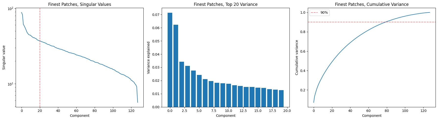

Finest Patches,: 80 components for 90% variance, top-1 explains 7.1%

cls_S, cls_U, cls_Vt, cls_var_exp = svd_analysis(enc_out2, level=0, title='CLS / Coarsest Patch,')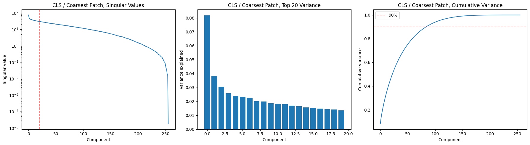

CLS / Coarsest Patch,: 85 components for 90% variance, top-1 explains 8.2%

Two key takeaways:

1. Patches need 178/256 dims for 90%. The representation is highly distributed with no dominant direction. This means the encoder is using nearly all its capacity, which is healthy (no dimensional collapse). But it also suggests rhythm and pitch aren’t cleanly factored — if they were, you’d expect a sharper elbow in the spectrum (the first 1 or 2 components notwithstanding).
2. CLS only needs 23/256 dims. The global summary is much more compressed. That’s interesting for generation: it suggests the “gist” of a musical passage lives in a ~23-dimensional subspace. The gradual slope in the top-20 bars (no single dominant component) means it’s not collapsing to a trivial representation either.

Decoder Performance

if cfg.model.get('encoder', 'vit') == 'swin': # decoder should match encoder
    decoder = SwinDecoder(img_height=cfg.data.image_size, img_width=cfg.data.image_size,
                        patch_h=cfg.model.patch_h, patch_w=cfg.model.patch_w,
                        embed_dim=cfg.model.embed_dim,
                        depths=cfg.model.get('dec_depths', cfg.model.depths), 
                        num_heads=cfg.model.get('dec_num_heads', cfg.model.num_heads)).to(device)
else: 
    decoder = ViTDecoder(cfg.data.in_channels, (cfg.data.image_size, cfg.data.image_size),
                     cfg.model.patch_size, cfg.model.dim, 
                     cfg.model.get('dec_depth', 4), cfg.model.get('dec_heads', 8)).to(device)

name = decoder.__class__.__name__
print("Name = ",name)
decoder = load_checkpoint(decoder, cfg.get('encoder_ckpt', f'../checkpoints/{decoder.__class__.__name__}__best.pt'))

Name =  SwinDecoder
>>> Loaded SwinDecoder checkpoint from ../checkpoints/SwinDecoder__best.pt

with torch.autocast(device_type='cpu', dtype=torch.bfloat16):
    recon_logits = decoder(enc_out2)
img_recon = torch.sigmoid(recon_logits).float().cpu() 
img_real = img2
print("img_recon.shape, img_real.shape =",img_recon.shape, img_real.shape)

img_recon.shape, img_real.shape = torch.Size([256, 1, 128, 128]) torch.Size([256, 1, 128, 128])

grid_recon, grid_real, grid_map, evals = viz_mae_recon(img_recon, img_real, enc_out=None, epoch=0, debug=False, return_maps=True)

fig, (ax1, ax2, ax3) = plt.subplots(1, 3, figsize=(10, 5))
ax1.imshow(grid_real.permute(1,2,0), cmap='gray'); ax1.set_title('Real')
ax2.imshow(grid_recon.permute(1,2,0), cmap='gray'); ax2.set_title('Recon')
ax3.imshow(grid_map.permute(1,2,0)); ax3.set_title('Map')
plt.show()
print(', '.join(f"{k}: {v.item():.4f}" for k, v in evals.items() if not k.endswith('map')))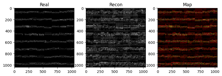

precision: 0.0978, recall: 0.3414, specificity: 0.8724, f1: 0.1521

In the next cell we’re gonna plot an image showing the maps as a very large image, we’re gonna hide it from the LLM because it doesn’t need to see it and we wanna spare the context.

img = Image.fromarray((grid_map*255).permute(1,2,0).byte().numpy())
display(img)

Pitch-time factorization

Cosine Histograms and PCA plots

batch_size = 256
ds = ShiftedTripletDataset(split='val')

subset = torch.utils.data.Subset(ds, range(batch_size * 10))  # 10 samples is enough
dl = DataLoader(subset, batch_size=batch_size, shuffle=False)
plt.close('all')
print("Collecting difference vectors...")
targets, schemes = [], []
for i, batch in enumerate(tqdm(dl)):
    img1, img2, img3 = batch['img1'], batch['img2'], batch['img3']
    deltas, scheme, target, scheme = batch['deltas'], batch['scheme'], batch['target'], batch['scheme']
    targets.append(target)
    schemes.append(scheme)
    with torch.no_grad(): 
        enc_out1 = encoder(img1)  # anchor
        enc_out2 = encoder(img2)  # crop 1
        enc_out3 = encoder(img3)  # crop 2 
    z1 = [lvl.emb for lvl in enc_out1.patches.levels]
    z2 = [lvl.emb for lvl in enc_out2.patches.levels]
    z3 = [lvl.emb for lvl in enc_out3.patches.levels]
    n_levels =  enc_out1.patches.num_levels

    # lazy-initialize the accumulation lists
    if i == 0: d2_vecs, d3_vecs = [[] for _ in range(n_levels)], [[] for _ in range(n_levels)]

    for lev in range(n_levels):
        d2, d3 = z2[lev]-z1[lev], z3[lev]-z1[lev] 
        d2, d3 = (z2[lev]-z1[lev]).mean(dim=1), (z3[lev]-z1[lev]).mean(dim=1) # mean pooling across patches
        d2_vecs[lev].append(d2)
        d3_vecs[lev].append(d3)
        
del dl
targets = torch.cat(targets,dim=0)
schemes = torch.cat(schemes,dim=0)

# print("Performing per-level analysis: (takes a while)")
# OUR_TARGET_NAMES = {-1.0: 'anti-parallel', 0.0: 'orthogonal', 1.0: 'parallel'}

# for lev in range(n_levels):
#     d2 = torch.cat(d2_vecs[lev], dim=0)
#     d3 = torch.cat(d3_vecs[lev], dim=0)
#     cos = F.cosine_similarity(d2, d3, dim=-1)
#     print(f"Level = {lev}:  d2 shape = {d2[lev].shape}, cos NaNs = {cos.isnan().sum()}")
#     n = min(len(cos), 20000)
#     idx = torch.randperm(len(cos))[:n]
#     cos_sub, targets_sub = cos[idx], targets[idx]
#     fig, ax = plt.subplots(1, 3, figsize=(8,2))
#     for i, (t_val, name)  in enumerate(OUR_TARGET_NAMES.items()):
#         mask = (targets_sub - t_val).abs() < 1e-3
#         ax[i].hist(cos_sub[mask].numpy().flatten(), bins=50, alpha=0.5, label=f"Level {lev}:\n N= {len(cos_sub[mask].numpy().flatten())}, {name}")
#         ax[i].set_ylabel('count')
#         ax[i].set_xlabel('cosine')
#         ax[i].set_xlim(-1, 1)
#         ax[i].legend(fancybox=True, framealpha=0.3)
#     plt.show()
#     plt.close()

Loading 91 val files from ~/datasets/POP909_images_basic/... Finished loading.
Collecting difference vectors...

from sklearn.decomposition import PCA

for lev in range(n_levels):
    d2 = torch.cat(d2_vecs[lev], dim=0)
    d3 = torch.cat(d3_vecs[lev], dim=0)

    # Separate into pitch and time diffs by scheme
    s0, s1, s2 = schemes == 0, schemes == 1, schemes == 2
    pitch_d = torch.cat([d2[s0], d3[s0], d2[s2]], dim=0)
    time_d  = torch.cat([d2[s1], d3[s1], d3[s2]], dim=0)

    all_diffs = torch.cat([pitch_d, time_d], dim=0).numpy()
    pca = PCA(n_components=2).fit(all_diffs)
    proj = pca.transform(all_diffs)
    n_pitch = len(pitch_d)

    fig, (ax1, ax2) = plt.subplots(1, 2, figsize=(12, 5))
    fig.suptitle(f'Level {lev}', fontsize=14)

    ax1.scatter(proj[:n_pitch, 0], proj[:n_pitch, 1], alpha=0.3, s=10, label='pitch Δ', c='blue')
    ax1.scatter(proj[n_pitch:, 0], proj[n_pitch:, 1], alpha=0.3, s=10, label='time Δ', c='green')
    ax1.set_xlabel('PC1'); ax1.set_ylabel('PC2'); ax1.legend()
    ax1.set_title('PCA of difference vectors'); ax1.set_aspect('equal')

    # Cross-type cosines
    n_min = min(len(pitch_d), len(time_d))
    cos_cross = F.cosine_similarity(pitch_d[:n_min], time_d[:n_min], dim=-1).numpy()

    # Same-type cosines by target
    same_type = s0 | s1
    par = same_type & (targets > 0.5)
    anti = same_type & (targets < -0.5)
    cos_par = F.cosine_similarity(d2[par], d3[par], dim=-1).numpy()
    cos_anti = F.cosine_similarity(d2[anti], d3[anti], dim=-1).numpy()

    ax2.hist(cos_cross, bins=40, alpha=0.5, label='pitch vs time (want ≈0)', density=True)
    ax2.hist(cos_par, bins=40, alpha=0.5, label='same-sign (want ≈+1)', density=True)
    ax2.hist(cos_anti, bins=40, alpha=0.5, label='opp-sign (want ≈−1)', density=True)
    ax2.set_xlabel('cosine similarity'); ax2.legend(); ax2.set_title('Cosine similarity distributions')

    plt.tight_layout()
    plt.show()
    plt.close()

    print(f"Level {lev}: cross={cos_cross.mean():.3f}, parallel={cos_par.mean():.3f}, anti={cos_anti.mean():.3f}\n")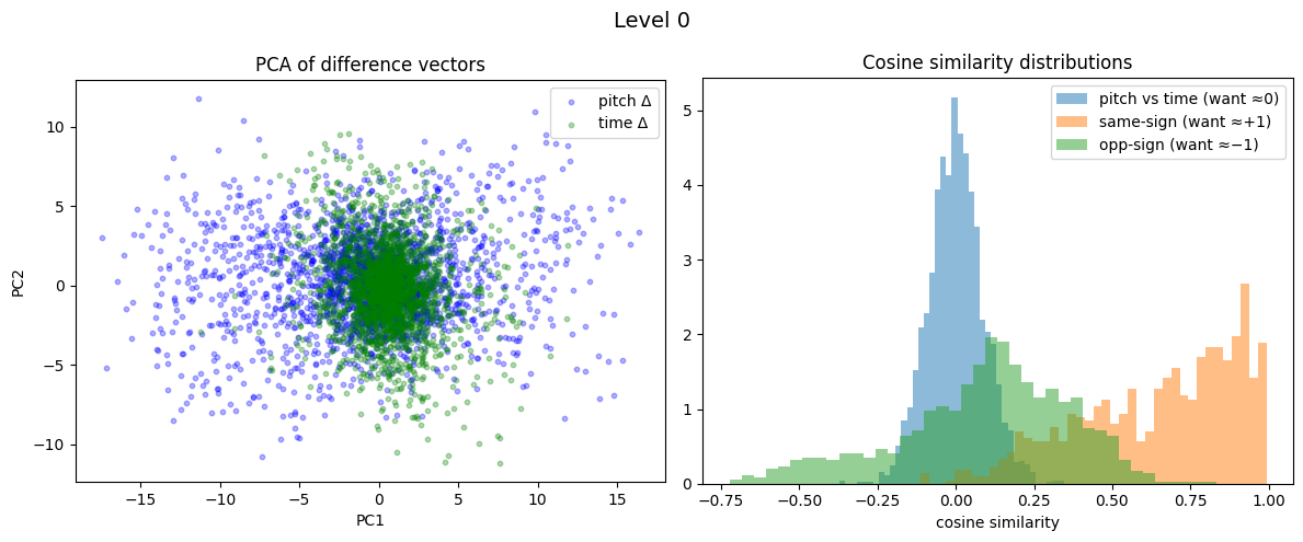

Level 0: cross=0.001, parallel=0.649, anti=0.092

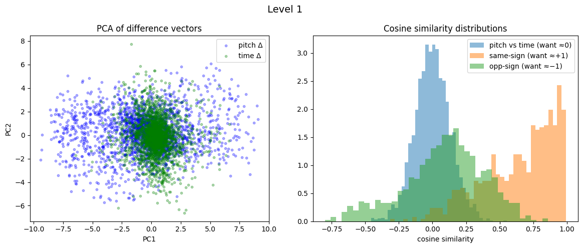
Level 1: cross=0.001, parallel=0.644, anti=0.089

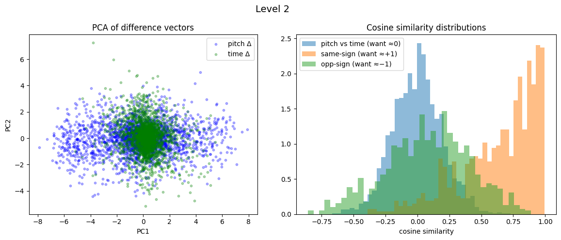
Level 2: cross=-0.003, parallel=0.639, anti=0.082

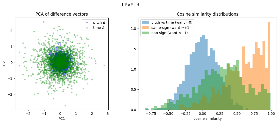
Level 3: cross=0.002, parallel=0.587, anti=0.280

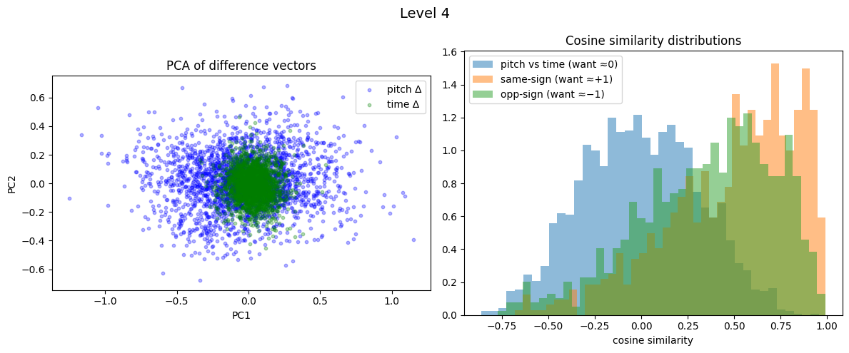
Level 4: cross=-0.005, parallel=0.491, anti=0.352

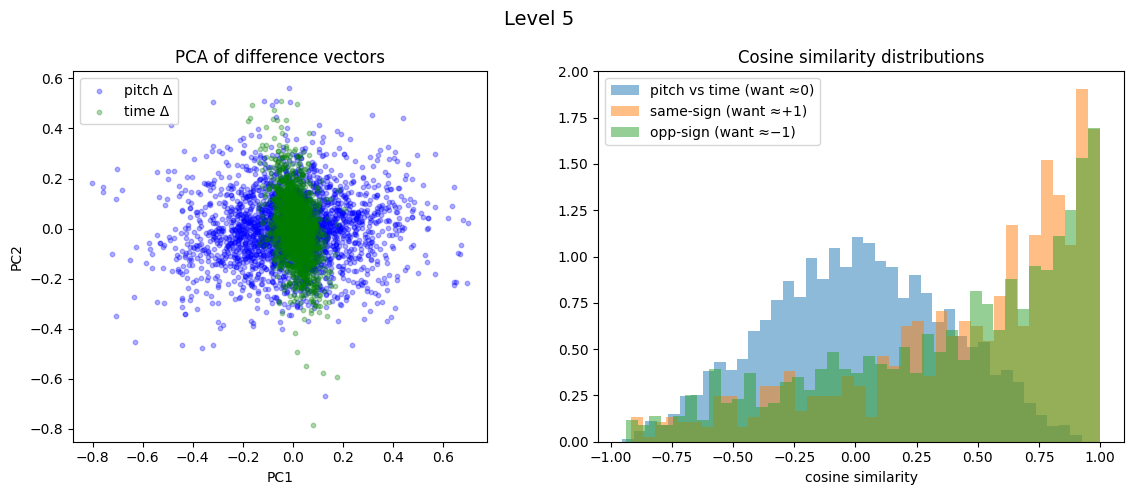
Level 5: cross=0.008, parallel=0.464, anti=0.389