b,d,n = 16,32,152
tokens = 2*torch.rand((b,d,n))-1
for bi in range(b):
mu = torch.rand((1,d,1)).tile((1,1,n))
tokens[bi,:,:] = mu + 0.7*tokens[bi,:,:]
layout_dict=dict( scene=dict( camera=dict( up=dict(x=0, y=0, z=1), eye=dict(x=0, y=2.0707, z=1), ), ) )
show_point_cloud(tokens, darkmode=True, layout_dict=layout_dict) # default, no lines connecting dotsviz
Vizualization routines
Originally written for https://github.com/zqevans/audio-diffusion/blob/main/viz/viz.py
embeddings_table
embeddings_table (tokens)
make a table of embeddings for use with wandb
proj_pca
proj_pca (tokens, proj_dims=3)
project_down
project_down (tokens, proj_dims=3, method='pca', n_neighbors=10, min_dist=0.3, debug=False, **kwargs)
this projects to lower dimenions, grabbing the first proj_dims dimensions
| Type | Default | Details | |
|---|---|---|---|
| tokens | batched high-dimensional data with dims (b,d,n) | ||
| proj_dims | int | 3 | dimensions to project to |
| method | str | pca | projection method: ‘pca’|‘umap’ |
| n_neighbors | int | 10 | umap parameter for number of neighbors |
| min_dist | float | 0.3 | umap param for minimum distance |
| debug | bool | False | print more info while running |
| kwargs |
3D Scatter plots
To visualize point clouds in notebook and on WandB:pca_point_cloud
pca_point_cloud (tokens, color_scheme='batch', output_type='wandbobj', mode='markers', size=3, line={'color': 'rgba(10,10,10,0.01)'}, **kwargs)
| Type | Default | Details | |
|---|---|---|---|
| tokens | embeddings / latent vectors. shape = (b, d, n) | ||
| color_scheme | str | batch | ‘batch’: group by sample, otherwise color sequentially |
| output_type | str | wandbobj | plotly | points | wandbobj. NOTE: WandB can do ‘plotly’ directly! |
| mode | str | markers | plotly scatter mode. ‘lines+markers’ or ‘markers’ |
| size | int | 3 | size of the dots |
| line | dict | {‘color’: ‘rgba(10,10,10,0.01)’} | if mode=‘lines+markers’, plotly line specifier. cf. https://plotly.github.io/plotly.py-docs/generated/plotly.graph_objects.scatter3d.html#plotly.graph_objects.scatter3d.Line |
| kwargs |
point_cloud
point_cloud (tokens, method='pca', color_scheme='batch', output_type='wandbobj', mode='markers', size=3, line={'color': 'rgba(10,10,10,0.01)'}, ds_preproj=1, ds_preplot=1, debug=False, colormap=None, darkmode=False, layout_dict=None, **kwargs)
returns a 3D point cloud of the tokens
| Type | Default | Details | |
|---|---|---|---|
| tokens | embeddings / latent vectors. shape = (b, d, n) | ||
| method | str | pca | projection method for 3d mapping: ‘pca’ | ‘umap’ |
| color_scheme | str | batch | ‘batch’: group by sample; integer n: n groups, sequentially, otherwise color sequentially by time step |
| output_type | str | wandbobj | plotly | points | wandbobj. NOTE: WandB can do ‘plotly’ directly! |
| mode | str | markers | plotly scatter mode. ‘lines+markers’ or ‘markers’ |
| size | int | 3 | size of the dots |
| line | dict | {‘color’: ‘rgba(10,10,10,0.01)’} | if mode=‘lines+markers’, plotly line specifier. cf. https://plotly.github.io/plotly.py-docs/generated/plotly.graph_objects.scatter3d.html#plotly.graph_objects.scatter3d.Line |
| ds_preproj | int | 1 | EXPERIMENTAL: downsampling factor before projecting (1=no downsampling). Could screw up colors |
| ds_preplot | int | 1 | EXPERIMENTAL: downsampling factor before plotting (1=no downsampling). Could screw up colors |
| debug | bool | False | print more info |
| colormap | NoneType | None | valid color map to use, None=defaults |
| darkmode | bool | False | dark background, white fonts |
| layout_dict | NoneType | None | extra plotly layout options such as camera orientation |
| kwargs |
To display in the notebook (and the online documenation), we need a bit of extra code:
show_pca_point_cloud
show_pca_point_cloud (tokens, color_scheme='batch', mode='markers', colormap=None, line={'color': 'rgba(10,10,10,0.01)'}, **kwargs)
display a 3d scatter plot of tokens in notebook
show_point_cloud
show_point_cloud (tokens, method='pca', color_scheme='batch', mode='markers', line={'color': 'rgba(10,10,10,0.01)'}, ds_preproj=1, ds_preplot=1, debug=False, **kwargs)
display a 3d scatter plot of tokens in notebook
| Type | Default | Details | |
|---|---|---|---|
| tokens | same arts as point_cloud | ||
| method | str | pca | |
| color_scheme | str | batch | |
| mode | str | markers | |
| line | dict | {‘color’: ‘rgba(10,10,10,0.01)’} | |
| ds_preproj | int | 1 | |
| ds_preplot | int | 1 | |
| debug | bool | False | |
| kwargs |
setup_plotly
setup_plotly (nbdev=True)
Plotly is already ‘setup’ on colab, but on regular Jupyter notebooks we need to do a couple things
on_colab
on_colab ()
Returns true if code is being executed on Colab, false otherwise
Test the point cloud viz inside a notebook:
Try UMAP:
show_point_cloud(tokens, method='umap') # default, no lines connecting dotsOr we can add lines connecting the dots, such as a faint gray line:
show_point_cloud(tokens, mode='lines+markers')And if we really want 2d instead of 3D, we can flatten to a pancake:
show_point_cloud(tokens, mode='lines+markers', method='umap', proj_dims=2)Print audio info
print_stats
print_stats (waveform, sample_rate=None, src=None, print=<built-in function print>)
print stats about waveform. Taken verbatim from pytorch docs.
Testing that:
audio_filename = 'examples/example.wav'
waveform = load_audio(audio_filename)
print_stats(waveform)Resampling examples/example.wav from 44100 Hz to 48000 Hz
Shape: (1, 55728)
Dtype: torch.float32
- Max: 0.647
- Min: -0.647
- Mean: 0.000
- Std Dev: 0.075
tensor([[-3.0239e-04, -3.8517e-04, -6.0043e-04, ..., 2.4789e-05,
-1.3458e-04, -8.0428e-06]])
Spectrograms
mel_spectrogram
mel_spectrogram (waveform, power=2.0, sample_rate=48000, db=False, n_fft=1024, n_mels=128, debug=False)
calculates data array for mel spectrogram (in however many channels)
spectrogram_image
spectrogram_image (spec, title=None, ylabel='freq_bin', aspect='auto', xmax=None, db_range=[35, 120], justimage=False, figsize=(5, 4))
Modified from PyTorch tutorial https://pytorch.org/tutorials/beginner/audio_feature_extractions_tutorial.html
| Type | Default | Details | |
|---|---|---|---|
| spec | |||
| title | NoneType | None | |
| ylabel | str | freq_bin | |
| aspect | str | auto | |
| xmax | NoneType | None | |
| db_range | list | [35, 120] | |
| justimage | bool | False | |
| figsize | tuple | (5, 4) | size of plot (if justimage==False) |
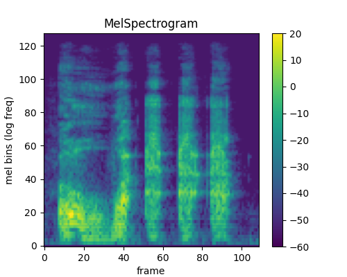
audio_spectrogram_image
audio_spectrogram_image (waveform, power=2.0, sample_rate=48000, print=<built-in function print>, db=False, db_range=[35, 120], justimage=False, log=False, figsize=(5, 4))
Wrapper for calling above two routines at once, does Mel scale; Modified from PyTorch tutorial https://pytorch.org/tutorials/beginner/audio_feature_extractions_tutorial.html
Let’s test the above routine:
spec_graph = audio_spectrogram_image(waveform, justimage=False, db=False, db_range=[-60,20])
display(spec_graph)/Users/shawley/envs/aa/lib/python3.10/site-packages/torchaudio/transforms/_transforms.py:611: UserWarning:
Argument 'onesided' has been deprecated and has no influence on the behavior of this module.
/Users/shawley/envs/aa/lib/python3.10/site-packages/torchaudio/functional/functional.py:576: UserWarning:
At least one mel filterbank has all zero values. The value for `n_mels` (128) may be set too high. Or, the value for `n_freqs` (513) may be set too low.
‘Playable Spectrograms’
Source(s): Original code by Scott Condron (@scottire) of Weights and Biases, edited by @drscotthawley
cf. @scottire’s original code here: https://gist.github.com/scottire/a8e5b74efca37945c0f1b0670761d568
and Morgan McGuire’s edit here; https://github.com/morganmcg1/wandb_spectrogram
playable_spectrogram
playable_spectrogram (waveform, sample_rate=48000, specs:str='all', layout:str='row', height=170, width=400, cmap='viridis', output_type='wandb', debug=True)
Takes a tensor input and returns a [wandb.]HTML object with spectrograms of the audio specs : “all_specs”, spectrograms only “all”, all plots “melspec”, melspectrogram only “spec”, spectrogram only “wave_mel”, waveform and melspectrogram only “waveform”, waveform only, equivalent to wandb.Audio object
Limitations: spectrograms show channel 0 only (i.e., mono)
| Type | Default | Details | |
|---|---|---|---|
| waveform | audio, PyTorch tensor | ||
| sample_rate | int | 48000 | sample rate in Hz |
| specs | str | all | see docstring below |
| layout | str | row | ‘row’ or ‘grid’ |
| height | int | 170 | height of spectrogram image |
| width | int | 400 | width of spectrogram image |
| cmap | str | viridis | colormap string for Holoviews, see https://holoviews.org/user_guide/Colormaps.html |
| output_type | str | wandb | ‘wandb’, ‘html_file’, ‘live’: use live for notebooks |
| debug | bool | True | flag for internal print statements |
generate_melspec
generate_melspec (audio_data, sample_rate=48000, power=2.0, n_fft=1024, win_length=None, hop_length=None, n_mels=128)
helper routine for playable_spectrogram
Sample usage with WandB:
wandb.init(project='audio_test')
wandb.log({"playable_spectrograms": playable_spectrogram(waveform)})
wandb.finish()See example result at https://wandb.ai/drscotthawley/playable_spectrogram_test/
Test the playable spectrogram. Let’s show off the multichannel waveform display:
mc_wave = load_audio('examples/stereo_pewpew.mp3')
playable_spectrogram(mc_wave, specs='wave_mel', output_type='live')Resampling examples/stereo_pewpew.mp3 from 44100.0 Hz to 48000 Hz