Crash Course On GANs

header-img

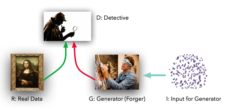
Image credit: Dev Nag

This post is not necessarily a crash course on GANs. It is at least a record of me giving myself a crash course on GANs. Adding to this as I go.

Intro/Motivation

I’ve been wanting to grasp the seeming-magic of Generative Adversarial Networks (GANs) since I started seeing handbags turned into shoes and brunettes turned to blondes… 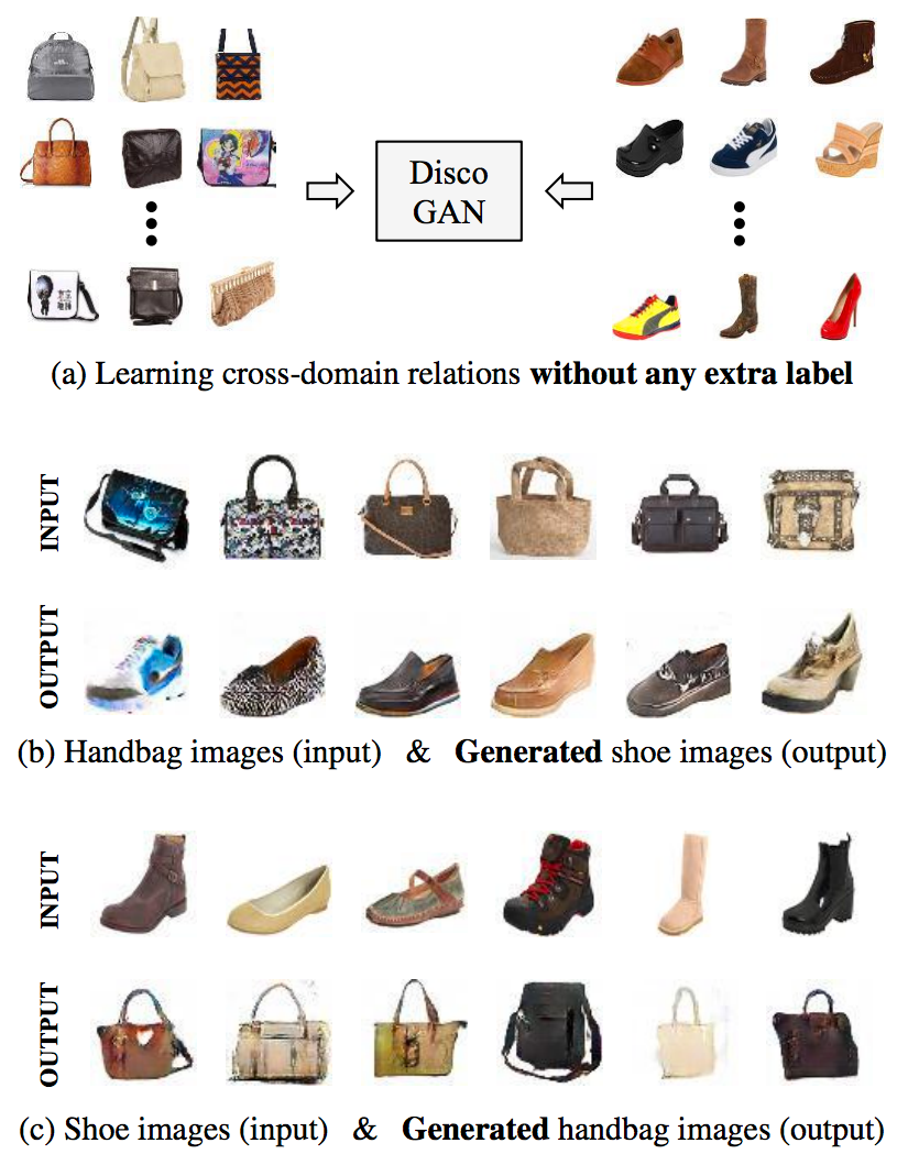…and seeing Magic Pony’s image super-resolution results and hearing that Yann Lecun had called GANs the most important innovation in machine learning in recent years.

Finally, seeing Google’s Cat-Pig Sketch-Drawing Math…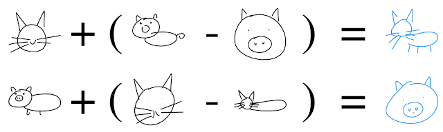

…broke me, and so…I need to ‘get’ this.

I’ve noticed that, although people use GANs with great success for images, not many have tried using them for audio yet (Note: see SEGAN paper, below). Maybe with already-successful generative audio systems like WaveNet, SampleRNN (listen to those piano sounds!!) and TacoTron there’s less of a push for trying GANs. Or maybe GANs just suck for audio. Guess I’ll find out…

Steps I Took

Day 1:

1. Gathered list of some prominent papers (below).
2. Watched video of Ian Goodfellow’s Berkeley lecture (notes below).
3. Started reading the EBGAN paper (notes below)…
4. …but soon switched to BEGAN paper – because wow! Look at these generated images:
5. Googled for Keras-based BEGAN implementations and other code repositories (below)…Noticed SEGAN…
6. …Kept reading BEGAN, making notes as I went (below).
7. Finished paper, started looking through BEGAN codes from GitHub (below) & began trying them out…
   1. Cloned @mokemokechicken’s Keras repo, grabbed suggested LFW database, converted images via script, ran training… Takes 140 seconds per epoch on Titan X Pascal.
   • Main part of code is in models.py
   2. Cloned @carpedm’s Tensorflow repo, looked through it, got CelebA dataset, started running code.
8. Leaving codes to train overnight. Next time, I’d like to try to better understand the use of an autoencoder as the discriminator.

Day 2:

1. My office is hot. Two Titan X GPUs pulling ~230W for 10 hours straight has put the cards up towards annoyingly high temperatures, as in ~ 85 Celsius! My previous nightly runs wouldn’t even go above 60 C. But the results – espically from the straight-Tensorflow code trained on the CelebA dataset – are as incredible as advertised! (Not that I understand them yet. LOL.) The Keras version, despite claiming to be a BEGAN implementation, seems to suffer from “mode collapse,” i.e. that too many very similar images get generated.
2. Fished around a little more on the web for audio GAN applications. Found an RNN-GAN application to MIDI, and found actual audio examples of what not to do: don’t try to just produce spectrograms with DCGAN and convert them to audio. The latter authors seem to have decided to switch to a SampleRNN approach. Perhaps it would be wise to heed their example? ;-)
3. Since EBGAN implemented autoencoders as discriminators before BEGAN did, I went back to read that part of the EBGAN paper. Indeed, section “2.3 - Using AutoEncoders” (page 4). (see notes below)
4. Ok, I basically get the autoencoder-discriminator thing now. :-)

Day 3:

“Life” intervened. :-/ Hope to pick this up later.

Papers

Haven’t read hardly any of these yet, just gathering them here for reference:

• Original GAN Paper: ” Generative Adversarial Networks” by GoodFellow (2014)

• DCGAN: “Unsupervised Representation Learning with Deep Convolutional Generative Adversarial Networks” by Radford, Metz & Chintala (2015)

• “Image-to-Image Translation with Conditional Adversarial Networks” by Isola et al (2016)

• “Improved Techniques for Training GANs” by Salimans et al (2016).

• DiscoGAN: “Learning to Discover Cross-Domain Relations with Generative Adversarial Networks” by Kim et al. (2017)

• EBGAN: “Energy-based Generative Adversarial Network by Zhao, Matheiu & Lecun (2016/2017).

  • Remarks/Notes:
  • “This variant [EBGAN] converges more stably [than previous GANs] and is both easy to train and robust to hyper-parameter variations” (quoting from BEGAN paper, below).
  • If it’s energy-based, does that mean we get a Lagrangian, and Euler-Lagrange Equations, and Lagrange Multipliers? And thus can physics students (& professors!) grasp these networks in a straightforward way? Should perhaps take a look at Lecun’s Tutorial on Energy-Based Learning.
  • “The energy is the resconstruction error [of the autoencoder]” (Section 1.3, bullet points)

  • 

    ebgan-pic

    Image credit: Roozbeh Farhoodi + EBGAN authors

  • “…256×256 pixel resolution, without a multi-scale approach.” (ibid)
  • Section 2.3 covers on the use of the autoencoder as a discriminator. Wow, truly, the discriminator’s “energy”/ “loss” criterion is literally just the reconstruction error of the autoencoder. How does that get you a discriminator??
  • It gets you a discriminator because the outputs of the generator are likely to have high energies whereas the real data (supposedly) will produce low energies: “We argue that the energy function (the discriminator) in the EBGAN framework is also seen as being regularized by having a generator producing the contrastive samples, to which the discrim- inator ought to give high reconstruction energies” (bottom of page 4).

• “Wasserstein GAN (WGAN) by Arjovsky, Chintala, & Bottou (2017)

• “BEGAN: Boundary Equilibrium Generative Adversarial Networks” by Berthelot, Schumm & Metz (April 2017).

  • Remarks/Notes:
  • “Our model is easier to train and simpler than other GANs architectures: no batch normalization, no dropout, no transpose convolutions and no exponential growth for convolution filters.” (end of section 3.5, page 5)
  • This is probably not the kind of paper that anyone off the street can just pick up & read. There will be math.
  • Uses an autoencoder for the discriminator.
  • I notice that Table 1, page 8 shows “DFM” (from “Improving Generative Adversarial Networks with Denoising Feature Matching” by Warde-Farley & Bengio, 2017) as scoring higher than BEGAN.
  • page 2: “Given two normal distributions…with covariances \[C_1, C_2\],…”: see “Multivariate Normal Distribution”.
  • Section 3.3, Equilibrium: The “\[\mathbb{E}[\ ]\]” notation – as in \[\mathbb{E}\left[\mathcal{L}(x)\right]\] – means “expected value.” See https://en.wikipedia.org/wiki/Expected_value
  • Introduces the diversity ratio: \[\gamma=\frac{\mathbb{E}\left[\mathcal{L}(G(z))\right]}{\mathbb{E}\left[\mathcal{L}(x)\right]}\]. “Lower values of \[\gamma\] lead to lower image diversity because the discriminator focuses more heavily on auto-encoding real images.”
  • “3.5 Model architecture”: Did not actually get the bit about the autoencoder as the discriminator: “How does an autoencoder output a 1 or a zero?”
    
  • Ok, done. Will come back later if needed; maybe looking at code will make things clearer…

• “SEGAN: Speech Enhancement Generative Adversarial Network” by Pascual, Bonafonte & Serra (April 2017). Actual audio GAN! They only used it to remove noise.

Videos

• Ian Goodfellow (original GAN author), Guest lecture on GANs for UC Berkeley CS295 (Oct 2016). 1 hour 27 minutes. NOTE: actually starts at 4:33. Watch at 1.25 speed.
  • Remarks/Notes:
  • This is on a fairly “high” level, which may be too much for some viewers; if hearing the words “probability distribution” over & over again makes you tune out, and e.g. if you don’t know what a Jacobian is, then you may not want to watch this.
  • His “Taxonomy of Generative Models” is GREAT!
  • The discriminator is just an ordinary classifier.
  • So, the generator’s cost function can be just the negative of the discriminator’s cost function, (i.e. it tries to “mess up” the discriminator), however that can saturate (i.e. produce small gradients) so instead they try to “maximize the probability that the discriminator will make a mistake” (44:12).
  • “KL divergence” is a measure of the ‘difference’ between two PD’s.
  • “Logit” is the inverse of the sigmoid/logistical function. (logit<–>sigmoid :: tan<–>arctan)
  • Jensen-Shannon divergence is a measure of the ‘similarity’ between two PD’s. Jensen-Shannon produces better results for GANs than KL/maximum likelihood.

Web Posts/Tutorials

• “Machine Learning is Fun Part 7: Abusing Generative Adversarial Networks to Make 8-bit Pixel Art” by Adam Geitgey, skip down to “How DCGANs Work” (2017)

• Post on BEGAN: https://blog.heuritech.com/2017/04/11/began-state-of-the-art-generation-of-faces-with-generative-adversarial-networks/

• An introduction to Generative Adversarial Networks (with code in TensorFlow)

• “Generative Adversarial Networks (GANs) in 50 lines of code (PyTorch)” by Dev Nag (2017)

• “Stability of Generative Adversarial Networks” by Nicholas Guttenberg (2016)

• “End to End Neural Art with Generative Models” by Bing Xu (2016)

• Kording Lab GAN Tutorial by Roozbeh Farhoodi :-). Nicely done, has code too.

Code

Keras:

• ‘Basic’ GAN with MNIST example: https://www.kdnuggets.com/2016/07/mnist-generative-adversarial-model-keras.html
• GAN, BiGAN & Adversarial AutoEncoder: https://github.com/bstriner/keras-adversarial
• Kording Lab’s GAN tutorial, Jupyter Notebook https://github.com/KordingLab/lab_teaching_2016/blob/master/session_4/Generative%20Adversarial%20Networks.ipynb. (Code is short and understandable.)
• Keras BEGAN:
  • https://github.com/mokemokechicken/keras_BEGAN: Only works on 64x64 images; BEGAN paper shows some 128x128
  • https://github.com/pbontrager/BEGAN-keras: No documentation, and I don’t see how it could run. I notice local variables being referenced in models.py as if they’re global.
• Keras DCGAN (MNIST): https://github.com/jacobgil/keras-dcgan
• Auxiliary Classifier GAN: https://github.com/lukedeo/keras-acgan

Tensorflow:

• BEGAN-Tensorflow: https://github.com/carpedm20/BEGAN-tensorflow
• EBGAN.Tensorflow: https://github.com/shekkizh/EBGAN.tensorflow
• SEGAN: https://github.com/santi-pdp/segan
• DCGAN-Tensorflow: https://github.com/carpedm20/DCGAN-tensorflow

PyTorch:

• Tutorial & simple implementation: https://github.com/devnag/pytorch-generative-adversarial-networks

Datasets

• CelebA: https://mmlab.ie.cuhk.edu.hk/projects/CelebA.html
• MNIST: https://yann.lecun.com/exdb/mnist/
• Speech enhancement: https://datashare.is.ed.ac.uk/handle/10283/1942
• “Labelled Faces in the Wild” https://vis-www.cs.umass.edu/lfw/

More References (Lists)

• “Delving deep into Generative Adversarial Networks (GANs): A curated list of state-of-the-art publications and resources about Generative Adversarial Networks (GANs) and their applications.”